Nowadays in the classrooms, in the courses of the economics’ undergraduate, the professors begin teaching the consumer theory, theme with big impact in Microeconomics. However, this theory is always taught without a pragmatic application in real life. Therefore, the article has the objective to introduce to the readers’ themes about applied economics in a programming language like Python.

In this article we use Python 3, also it is necessary to install the libraries numpy, matplotlib, and scipy as we show in the next code:

1
2
3

import numpy as np
import matplotlib.pyplot as plt
from scipy.optimize import minimize

We import the NumPy library because we will need it to simplify the function expressions in Python. In addition, we import the matplotlib.pyplot library to make the function graphs, explained later, related to the utility function of goods. Finally, we use the scipy.optimize library to optime the utility function with the SLSQP method, as an example.

Consumer Theory

The consumer theory is the branch of the economy in charge of analyzing the economic agents’ behavior, specifically how they designate their wages in goods purchase to obtain the mayor welfare as possible.

We take into account the neoclassic theory of the consumers based on the preferences of the economic agent and his budget constraint.

Utility Function

It is the function that designates a utility level (or welfare) to a bucket of goods in the market, based on the preferences of the economic agent. These are some example of utility: functions:

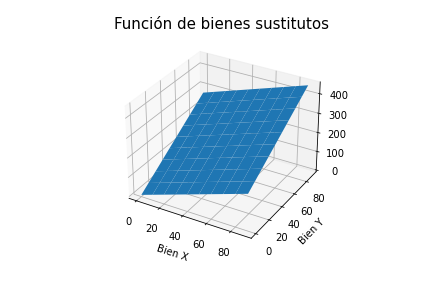
• Substitutes goods function:

In this case, two goods (X, Y) are perfect substitutes if the consumer is disposed to substitute a good for another at a constant rate.

1
2
3
4
5
6
7
8
9
10
11
12
13

x=y=np.arange(0.0, 100, 10)
X, Y=np.meshgrid(x,y)
def funcion_objetivo(x,y):
    a=2
    b=3
    return(x*(a)+y*(b))
fig=plt.figure()
ax=fig.gca(projection='3d')
ax.plot_surface(X,Y, funcion_objetivo(X,Y))
ax.set_ylabel("Bien Y")
ax.set_xlabel("Bien X")
ax.set_title("Función de bienes sustitutos", fontsize=15)
plt.savefig('sustitutos.png')

• Cuasi-linear function:

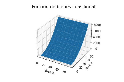
For this case, the X good is lineal, therefore the Y good depends only on the price relation (p1/p2) and not on the consumer’s wage like X does.

1
2
3
4
5
6
7
8
9
10

x=y=np.arange(0.0, 100, 10)
X, Y=np.meshgrid(x,y)
Z=X+Y**2
fig=plt.figure()
ax=fig.gca(projection='3d')
ax.plot_surface(X,Y, Z)
ax.set_ylabel("Bien Y")
ax.set_xlabel("Bien X")
ax.set_title("Función de bienes cuasilineal", fontsize=15)
plt.savefig('cuasilineal.png')

• Cobb-Douglas Function:

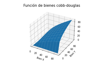
The total of the exponents must be one to find a global solution in the optimization, which is a feature of this function.

1
2
3
4
5
6
7
8
9
10
11
12
13

x=y=np.arange(0.0, 100, 10)
X, Y=np.meshgrid(x,y)
def funcion_objetivo(x,y):
    alfa=2/3
    beta=1/3
    return(x**(alfa)*y**(beta))
fig=plt.figure()
ax=fig.gca(projection='3d')
ax.plot_surface(X,Y, funcion_objetivo(X,Y))
ax.set_ylabel("Bien Y")
ax.set_xlabel("Bien X")
ax.set_title("Función de bienes cobb-douglas", fontsize=15)
plt.savefig('cobb.png')

Consumer choice:

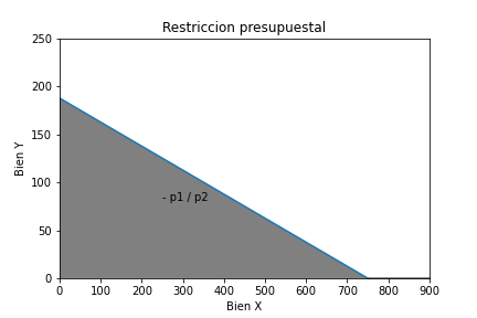
The consumer has to choose the bucket goods that maximize his welfare, in this case, utility, subject to budget constrain based on the market prices and his wage.

The consumer has to use his wage at least:

This is the case for two goods.

Therefore, the budget constraint used in the consumer’s optimization is the following:

Where W is “wage”.

1
2
3
4
5
6
7
8
9
10
11
12
13
14
15

x=np.arange(0.0, 1000, 10)
w=1500
p=[2,8]
y=w/p[1]-(p[0]*x/p[1])
plt.plot(x,y)
#plt.plot(sol.x)
plt.ylim([0,250])
plt.xlim([0,900])
plt.xlabel("Bien X")
plt.ylabel("Bien Y")
plt.title("Restriccion presupuestal")
plt.text(250, 80, "- p1 / p2")
plt.fill_between(x, y,1, color="grey")
plt.show()
plt.savefig('restriccion.png')

In addition, based on the assumption of not satiability in the economic agent preferences, the budget set becomes in a budget line that also contains the basket of goods where the cost is equal to the wage. $ p_xX+p_yY=W$ So, the consumer election problem is summarized in the following maximization:

The following function is the example of the maximization of the Cobb-Dougglas function made in Python:

Most of the optimization programs compute only the minimization of the functions. We need to convert the objective function into a negative function as we describe as follows, to obtain the result of the maximization.

1
2
3
4
5
6
7
8
9
10
11
12
13
14

def restriccion_1(x):
    w=1500
    p=[2,8]
    return -w+p[0]*x[0]+p[1]*x[1]
def objetivo(X):
    x,y=X
    alpha=2/3
    beta=1/3
    return -(x**(alpha)*y**(beta))
b=(0,None)
bnds=(b,b)
restriccion=[{'type':'eq', 'fun':restriccion_1}]
sol=minimize(objetivo, (0,0), method="SLSQP", constraints=restriccion, bounds=bnds)
optimo=sol.x

The analytical solution of this problem is a tuple (X = 500, Y = 62.5). However, Python returns a numeric solution (X = 499,9 y Y = 62,5) which is very close to the analytical solution. The following graph is the numeric solution:

1
2
3
4
5
6
7
8
9
10
11
12
13
14
15
16
17
18
19
20
21
22
23

x=y=np.arange(0.0, 1000,10)
X,Y=np.meshgrid(x,y)
def func_(f,X,Y):
    s=np.shape(X)
    return f(np.vstack([X.ravel(),Y.ravel()])).reshape(*s)
def objetivo(X):
    x,y=X
    alpha=2/3    
    beta=1/3
    return (x**(alpha)*y**(beta))
w=1500
p=[2,8]
fig, ax=plt.subplots(figsize=(8,6))
c=ax.contour(X,Y, func_(objetivo,X,Y), 40)
ax.plot(optimo[0], optimo[1], "b*")
ax.plot(x, w/p[1]-(p[0]*x/p[1]))
ax.fill_between(x, w/p[1]-(p[0]*x/p[1]),1, color='grey') 
ax.set_ylim(0, 300)
ax.text(optimo[0], optimo[1], "%s, %s"%(optimo[0], optimo[1]))
ax.set_ylabel("Bien Y")
ax.set_xlabel("Bien X")
ax.set_title("Optimo", fontsize=15)
plt.savefig("optimo.png")

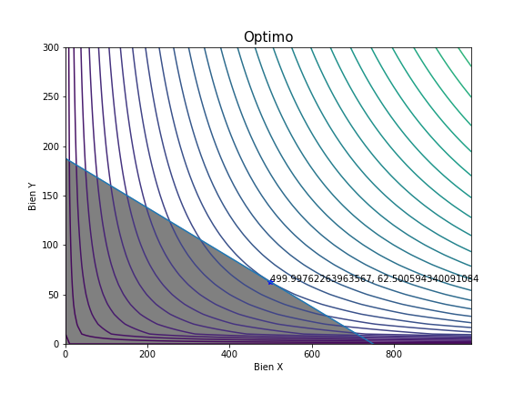
As we can see, the economic theory that taught day by day in the university cloisters can be didactic with a new point of view related to computer programming. Thus, this article invites readers to delve into the world of programming, which will help make professional training more comprehensive to the labor market.

References:

• Guerrera, J., Sánchez, A. & Zambrano, A. (2006). Notas de Microeconomía I.
• Carvajal, A., Riascos, A. (2012). Introducción a la Teoría Micreconómica.
• http://www.eco.uc3m.es/docencia/microeconomia/Transparencias/M1.pdf.
• http://allman.rhon.itam.mx/~aburto/eco%203/Preferencias_y_utilidad_del_consumidor_2010_a.pdf.